
Fișier:Mandelbrot set Components.jpg
Mărește rezoluția imaginii (1.000 × 1.000 pixeli, mărime fișier: 69 KB, tip MIME: image/jpeg)
| Acest fișier se află la Wikimedia Commons. Consultați pagina sa descriptivă acolo. |

|
O versiune vectorială a acestei imagini (SVG) este disponibilă.
Aceasta ar trebui folosită în locul vechii imagini pentru o afișare mai bună la rezoluții mari. File:Mandelbrot set Components.jpg → File:Mandelbrot Components.svg
Pentru mai multe informații despre imaginile vectoriale, consultați pagina Commons transition to SVG. Vedeți, de asemenea, și informațiile despre modul în care software-ul MediaWiki acceptă imagini în format SVG. |
 |
Descriere fișier
| Descriere |
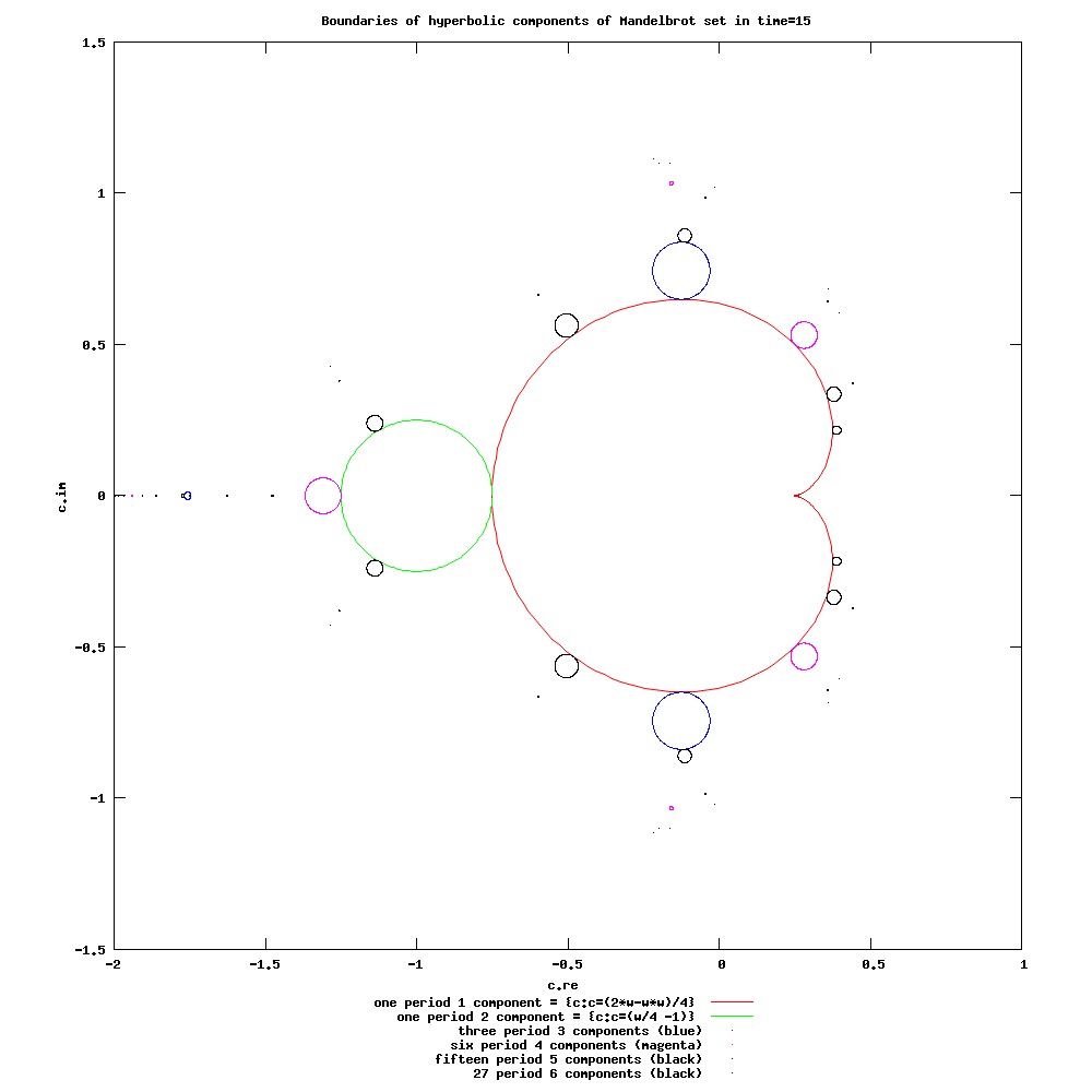
English: Boundaries of 53 hyperbolic components of Mandelbrot set for periods 1-6 made with polynomial maps from the unit circle Polski: Brzeg składowych zbioru Mandelbrot obliczony na podstawie równań brzegowych |
| Dată | |
| Sursă | Own work by uploader in Maxima and Gnuplot with help of many people ( see references ) |
| Autor | Adam majewski |
Description with Maxima code
Boundaries of hyperbolic components of Mandelbrot sets are closed curves : cardioids[1] or circles.
Douady-Hubbard-Sullivan theorem (DHS) states that unit circle can be mapped to boundary of hyperbolic component. This relation id defined by boundary equations. Here these equations, are used to draw boundaries of hyperbolic components.
Douady-Hubbard-Sullivan theorem
Douady-Hubbard-Sullivan theorem (DHS) states that the multiplier map " of an attracting periodic orbit is a conformal isomorphism from a hyperbolic component of the Mandelbrot set onto the unit disk and it extends homeomorpically to the boundaries." [2]


Here it is important that it maps boundary of hyperbolic component to boundary of unit disk ( = unit circle ) :

and it's inverse function maps unit circle to boundary of hyperbolic components :

The algorithm
The algorithm consist of 2 big steps :
- rasterisation of closed curve parametrised by angle
- complex mapping.

In datails there are more steps.
For given period do steps :

- Decide how many points of closed curve you want to draw ( iMax ).
- Compute
- start with
- while repeat :
- compute point of the unit circle in the standard plane where is an internal angle,
- map points onto the parameter plane (complex mapping ) using one of 2 methods :
- using explicit function ( it is possible only for periods 1-3)
- solving implicit equation with respect to ( it is posible for periods 1-8 using numerical methods)
- compute new angle


- draw set of points, which looks like curve [3]
Relations between hyperbolic components and unit circle
Definitions
f(z,c):=z*z+c;
F(n, z, c) :=
   if n=1 then f(z,c)
   else f(F(n-1, z, c),c);
Multiplier of periodic orbit :

_lambda(n):=diff(F(n,z,c),z,1);
Unit circle = boundary of unit disk


where coordinates of point of unit circle in exponential form are :


Boundary equations
Boundary equation

- defines relations between hyperbolic components and unit circle for given period ,
- allows computation of exact coordinates of hyperbolic componenets.
is boundary polynomial ( implicit function of 2 variables ).

Equations are in papers of Brown[4],John Stephenson[5], Wolf Jung[6]. Methods of finding boundary equations are also described in WikiBooks.
For boundary points :

so boundary equations can be in 4 equivalent forms :
| period | exponential | trigonometric | ||
|---|---|---|---|---|
| 1 | ||||
| 2 |


For higher periods only P-form is used, because it is the shortest and usefull for computations.
for period 3 :

for period 4 :

for period 5 :

Solving boundary equations with respect to c
Boundary equations for periods:
- 1-3 it can be solved with symbolical methods and give explicit solution :
- 1-2 it is easy to solve [7]
- 3 it can be solve using "elementary algebra" ( Stephenson )
- >3 it can't be solved explicitly and must be solved numerically with respect to .
period 1

There is only one period 1 component. [8] Because boundary equation is simple :
so it is easy to get inverse multiplier map :

For each internal angle one computes :
- point on unit circle ,
- point


Result is a list of boundary points .
period 2
Because boundary equation is simple :
so it is easy to get inverse multiplier map :

For each internal angle one computes :
- point on unit circle ,
- point


Result is a list of boundary points .
period 3

There are 3 period 3 components[9] Here solution of boundary equation gives 3 inverse multiplier maps .

It is possible in 3 ways :
- Munafo method[10] (every functions maps one half of one component and one half of other component)
- Giarrusso-Fisher method [11] ( one function for one component )
- Walter Hannah method
I use functions by Robert Munafo.
(%i3) b3:c^3+2*c^2+(1-P)*c+(P-1)^2=0$
(%i4) solve(b3,c);
(%o4) [
c=(-(sqrt(3)*%i)/2-1/2)*(((P-1)*sqrt(27*P^2-22*P+23))/(6*sqrt(3))-(27*P^2-36*P+25)/54)^(1/3)+
(((sqrt(3)*%i)/2-1/2)*(3*P+1))/(9*(((P-  1)*sqrt(27*P^2-22*P+23))/(6*sqrt(3))-(27*P^2-36*P+25)/54)^(1/3))-2/3,
c=((sqrt(3)*%i)/2-1/2)*
(((P-1)*sqrt(27*P^2-22*P+23))/(6*sqrt(3))-(27*P^2-36*P+25)/54)^(1/3)+
((-(sqrt(3)*%i)/2-1/2)*(3*P+1))/(9*(((P-1)*sqrt(27*P^2-22*P+23)) /(6*sqrt(3))-
(27*P^2-36*P+25)/54)^(1/3))-2/3,
c=(((P-1)*sqrt(27*P^2-22*P+23))/(6*sqrt(3))-(27*P^2-36*P+25)/54)^(1/3)+
(3*P+1)/(9*(((P-1)*sqrt(27*P^2-22*P+23))/(6*sqrt(3))-(27*P^2-36*P+25)/54)^(1/3))
For each internal angle one computes :
- point on unit circle ,
- points :


Result is a list of boundary points .
period 4
Boundary equation one can find in Mu-Ency. It can't be solved symbolicaly so it must be evaluated numerically [12].

It is 1 equation with 2 variables. To solve it one has to compute and put in . Now it is equation with 1 variable and it can be solved numerically.

For each internal angle one computes :
- point on unit circle ,
- Boundary polynomial
- solve boundary equation with respect to . Result is 6 roots ( each for one of 6 period 4 components).


Result is a list of boundary points .
b4(w):=c^6 + 3*c^5 + (w/16+3)* c^4 + (w/16+3)* c^3  - (w/16+2)* (w/16-1)* c^2 - (w/16-1)^3;
l(t):=%e^(%i*t*2*%pi);
iMax:200; /* number of point */
dt:1/iMax;
/* point to point method of drawing */
t:0; /* angle in turns */
w:rectform(ev(l(t), numer)); /* "exponential form prevents allroots from working", code by Robert P. Munafo */
/* compute equation for given w */
per4:expand(b4(w));
/* compute 6 complex roots and save them to the list cc4 */
cc4:allroots(per4);
/*  create new lists and save coordinates  to draw it later */
xx4:makelist (realpart(rhs(cc4[1])), i, 1, 1);
yy4:makelist (imagpart(rhs(cc4[1])), i, 1, 1);
for j:2 thru 6 step 1 do
 block
 (
  xx4:cons(realpart(rhs(cc4[j])),xx4),
  yy4:cons(imagpart(rhs(cc4[j])),yy4)
 );
for i:2 thru iMax step 1 do
block
( t:t+dt,
  w:rectform(ev(l(t), numer)), /* code by Robert P. Munafo  */
  per4:expand(m4(w)),
  cc4:allroots(per4),
  for j:1 thru 6 step 1 do
   block
   (
    xx4:cons(realpart(rhs(cc4[j])),xx4),
    yy4:cons(imagpart(rhs(cc4[j])),yy4)
   )
  );
period 5
one computes in the same way as for period 4, only implicit function is diffrent and there are 15 components.
period 6
one computes in the same way as for period 4, only implicit function is diffrent (see Stephenson paper II ) and there are 27 components.
period 7
one computes in the same way as for period 4, only implicit function is diffrent (degree in c is 63; see Stephenson paper III ) and there are 63 components.
period 8
Implicit equation can be computed but "is too large to exhibit" (see Stephenson paper III ). There are 120 components.

Higher periods
"Although extension of the arithmethic method to higher orders is possible in principle, the computations become to big in space and time " (Stephenson paper III )
Relations between boundary equation, multiplier map, inverse multiplier map and multiplier
| period | ||||
|---|---|---|---|---|
| 1 | ||||
| 2 | ||||
| 3 |


Symbolic solution of boundary equation is possible only for periods 1-3 ( with respect to or ). Every function can be in 4 equivalent forms : P, w, exponential t, trigonometric t (see boundary equations for details).
Period 1
Solving with respect to gives 2 results. hoose attracting one.
Period 2
Solving is simple because these are degree 1 equations ( with respect to both and ).
Period 3
Solving with respect to is possible in 3 ways.
Solving with respect to gives 2 results. One have to choose attracting.
Maxima source code
/*
batch file for Maxima
http://maxima.sourceforge.net/
wxMaxima 0.7.6 http://wxmaxima.sourceforge.net archive copy at the Wayback Machine
Maxima 5.16.1 http://maxima.sourceforge.net
Using Lisp GNU Common Lisp (GCL) GCL 2.6.8 (aka GCL)
Distributed under the GNU Public License.
based on :
http://www.mrob.com/pub/muency/brownmethod.html
*/
start:elapsed_run_time ();
iMax:200; /* number of points to draw */
dt:1/iMax;
/*
unit circle D={w:abs(w)=1 } where w=l(t)
t is angle in turns ; 1 turn = 360 degree = 2*Pi radians
*/
l(t):=%e^(%i*t*2*%pi);
/*
conformal maps from unit circle
to hyperbolic component of Mandelbrot set of period 1-4
These functions ( maps ) are computed in other batch file
*/
/* ---------------  inverse function of multiplier map : explicit function : c=gamma_p(P)  where P = w/(2^period) ---------------- */
gamma1(P):=P-P^2;
gamma2(P):=P - 1;
/* code of functions by Robert P. Munafo */
gamma3a(P):=(-(sqrt(3)*%i)/2-1/2)*(((P-1)*sqrt(27*P^2-22*P+23))/(6*sqrt(3))-(27*P^2-36*P+25)/54)^(1/3)+
(((sqrt(3)*%i)/2-1/2)*(3*P+1))/(9*(((P-1)*sqrt(27*P^2-22*P+23))/(6*sqrt(3))-(27*P^2-36*P+25)/54)^(1/3))-2/3;
gamma3b(P):=((sqrt(3)*%i)/2-1/2)*(((P-1)*sqrt(27*P^2-22*P+23))/(6*sqrt(3))-(27*P^2-36*P+25)/54)^(1/3)+
((-(sqrt(3)*%i)/2-1/2)*(3*P+1))/(9*(((P-  1)*sqrt(27*P^2-22*P+23))/(6*sqrt(3))-(27*P^2-36*P+25)/54)^(1/3))-2/3;
gamma3c(P):=(((P-1)*sqrt(27*P^2-22*P+23))/(6*sqrt(3))-(27*P^2-36*P+25)/54)^(1/3)+(3*P+1)/(9*(((P-1)*sqrt(27*P^2-22*P+23))/
(6*sqrt(3))-   (27*P^2-36*P+25) /54)^(1/3))-2/3;
/* ---------- boundary equation (implicit function)  b_p(P,c)=0 ------------------------------------------------------------------ */
b4(P):=c^6 + 3*c^5 + (P+3)* c^4 + (P+3)* c^3  - (P+2)*(P-1)*c^2 - (P-1)^3;
/* ------ period 5 ------------- */
b5(P):=c^15 +
8*c^14 +
28*c^13 +
(P + 60)*c^12 +
(7*P + 94)*c^11 +
(3*(P)^2 + 20*P + 116)*c^10 +
(11*P^2 + 33*P + 114)*c^9 +
(6*P^2 + 40*P + 94)*c^8 +
(2*P^3 - 20*P^2 + 37*P + 69)*c^7 +
(3*P - 11)*(3*P^2 - 3*P - 4)*c^6 +
(P - 1)*(3*P^3 + 20*P^2 - 33*P - 26)*c^5 +
( 3*P^2 + 27*P + 14)*((P - 1)^2)*c^4 -
(6*P + 5)*((P - 1)^3 )*c^3 +
(P + 2)*((P - 1)^4)*c^2 -
c*(P - 1)^5  +
(P - 1)^6 ;
/*-----period 6 ----------------------- */
b6(P):=
c^27+
13*c^26+
78*c^25+
(293 - P)*c^24+
(792 - 10*P)*c^23+
(1672 - 41*P)*c^22+
(2892 - 84*P - 4*P^2)*c^21+
(4219 - 60*P - 30*P^2)*c^20+
(5313 + 155*P - 80*P^2)*c^19+
(5892 + 642*P - 57*P^2 + 4*P^3)*c^18+
(5843 + 1347*P + 195*P^2 + 22*P^3)*c^17+
(5258 + 2036*P + 734*P^2 + 22*P^3)*c^16+
(4346 + 2455*P + 1441*P^2 - 112*P^3 + 6*P^4)*c^15 +
(3310 + 2522*P + 1941*P^2 - 441*P^3 + 20*P^4)*c^14 +
(2331 + 2272*P + 1881*P^2 - 853*P^3 - 15*P^4)*c^13 +
(1525 + 1842*P + 1344*P^2 - 1157*P^3 - 124*P^4 - 6*P^5)*c^12 +
(927 + 1385*P + 570*P^2 - 1143*P^3 - 189*P^4 - 14*P^5)*c^11 +
(536 + 923*P - 126*P^2 - 774*P^3 - 186*P^4 + 11*P^5)*c^10 +
(298 + 834*P + 367*P^2 + 45*P^3 - 4*P^4 + 4*P^5)*(1-P)*c^9 +
(155 + 445*P - 148*P^2 - 109*P^3 + 103*P^4 + 2*P^5)*(1-P)*c^8 +
2*(38 + 142*P - 37*P^2 - 62*P^3 + 17*P^4)*(1-P)^2*c^7 +
(35 + 166*P + 18*P^2 - 75*P^3 - 4*P^4)*((1-P)^3)*c^6 +
(17 + 94*P + 62*P^2 + 2*P^3)*((1-P)^4)*c^5 +
(7 + 34*P + 8*P^2)*((1-P)^5)*c^4 +
(3 + 10*P + P^2)*((1-P)^6)*c^3 +
(1 + P)*((1-P)^7)*c^2 +
-c*((1-P)^8) + (1-P)^9;
/*-----------------------------------*/
/* point to point method of drawing */
t:0; /* angle in turns */
/* compute first point of curve, create list and save point to this list */
/* point of unit circle   w:l(t); */
w:rectform(ev(l(t), numer)); /* "exponential form prevents allroots from working", code by Robert P. Munafo */
/* ---- period 1 -------------------*/
P:w/2;
c1:gamma1(P);
xx1:makelist (realpart(c1), i, 1, 1); /* save coordinates  to draw it later */
yy1:makelist (imagpart(c1), i, 1, 1);
/* -----period 2 --------------*/
P:P/2;
c2:gamma2(P);
xx2:makelist (realpart(c2), i, 1, 1);
yy2:makelist (imagpart(c2), i, 1, 1);
/* period 3 components */
P:P/2;
c3:gamma3a(P);
xx3a:makelist (realpart(c3), i, 1, 1);
yy3a:makelist (imagpart(c3), i, 1, 1);
c3:gamma3b(w);
xx3b:makelist (realpart(c3), i, 1, 1);
yy3b:makelist (imagpart(c3), i, 1, 1);
c3:gamma3c(w);
xx3c:makelist (realpart(c3), i, 1, 1);
yy3c:makelist (imagpart(c3), i, 1, 1);
/* period 4 */
P:P/2;
per4:expand(b4(P)); /* compute equation for given w ( t) */
cc4:allroots(per4); /* compute 6 complex roots and save them to the list cc4 */
/*  create new lists and save coordinates  to draw it later */
xx4:makelist (realpart(rhs(cc4[1])), i, 1, 1);
yy4:makelist (imagpart(rhs(cc4[1])), i, 1, 1);
for j:2 thru 6 step 1 do
block
(
xx4:cons(realpart(rhs(cc4[j])),xx4),
yy4:cons(imagpart(rhs(cc4[j])),yy4)
);
/* period 5 */
P:P/2;
per5:expand(b5(P)); /* compute equation for given w ( t) */
cc5:allroots(per5); /* compute 15 complex roots and save them to the list cc5 */
/*  create new lists and save coordinates  to draw it later */
xx5:makelist (realpart(rhs(cc5[1])), i, 1, 1);
yy5:makelist (imagpart(rhs(cc5[1])), i, 1, 1);
for j:2 thru 15 step 1 do
block
(
xx5:cons(realpart(rhs(cc5[j])),xx5),
yy5:cons(imagpart(rhs(cc5[j])),yy5)
);
/* period 6 */
P:P/2;
per6:expand(b6(P)); /* compute equation for given w ( t) */
cc6:allroots(per6); /* compute 15 complex roots and save them to the list cc5 */
/*  create new lists and save coordinates  to draw it later */
xx6:makelist (realpart(rhs(cc6[1])), i, 1, 1);
yy6:makelist (imagpart(rhs(cc6[1])), i, 1, 1);
for j:2 thru 27 step 1 do
block
(
 xx6:cons(realpart(rhs(cc6[j])),xx6),
 yy6:cons(imagpart(rhs(cc6[j])),yy6)
) ;
/* ------------*/
for i:2 thru iMax step 1 do
block
( t:t+dt,
 w:rectform(ev(l(t), numer)), /* "exponential form prevents allroots from working", code by Robert P. Munafo */
 P:w/2,
 c1:gamma1(P),
 /* save values to draw it later */
 xx1:cons(realpart(c1),xx1),
 yy1:cons(imagpart(c1),yy1),
 P:P/2,
 c2:gamma2(P),
 xx2:cons(realpart(c2),xx2),
 yy2:cons(imagpart(c2),yy2),
 P:P/2,
 c3:gamma3a(P),
 xx3a:cons(realpart(c3),xx3a),
 yy3a:cons(imagpart(c3),yy3a),
 c3:gamma3b(P),
 xx3b:cons(realpart(c3),xx3b),
 yy3b:cons(imagpart(c3),yy3b),
 c3:gamma3c(P),
 xx3c:cons(realpart(c3),xx3c),
 yy3c:cons(imagpart(c3),yy3c),
 /* period 4 */
 P:P/2,
 per4:expand(b4(P)),
 cc4:allroots(per4),
 for j:1 thru 6 step 1 do
  block
   (
   xx4:cons(realpart(rhs(cc4[j])),xx4),
   yy4:cons(imagpart(rhs(cc4[j])),yy4)
   ),
 /* period 5 */
 P:P/2,
 per5:expand(b5(P)), /* compute equation for given w ( t) */
 cc5:allroots(per5), /* compute 15 complex roots and save them to the list cc5 */
 for j:1 thru 15 step 1 do
 block
  (
  xx5:cons(realpart(rhs(cc5[j])),xx5),
  yy5:cons(imagpart(rhs(cc5[j])),yy5)
  ),
 /* period 6 */
 P:P/2,
 per6:expand(b6(P)), /* compute equation for given w ( t) */
 cc6:allroots(per6), /* compute 27 complex roots and save them to the list cc6 */
 for j:1 thru 27 step 1 do
  block
  (
  xx6:cons(realpart(rhs(cc6[j])),xx6),
  yy6:cons(imagpart(rhs(cc6[j])),yy6)
  )
 );
stop:elapsed_run_time ();
time:fix(stop-start);
load(draw);
draw2d(
  file_name = "", /* file in directory  C:\Program Files\Maxima-5.16.1\wxMaxima */
  terminal  = 'screen, /* jpg when draw to file with jpg extension */
  pic_width  = 1000,
  pic_height = 1000,
  yrange = [-1.5,1.5],
  xrange = [-2,1],
  title= concat("Boundaries of 53 hyperbolic components of Mandelbrot set made in ",string(time),"sec"),
  xlabel     = "c.re ",
  ylabel     = "c.im",
  point_type    = dot,
  point_size    = 5,
  points_joined =true,
  user_preamble="set size square;set key out vert;set key bot center",
  key = "one period 1 component = {c:c=(2*w-w*w)/4} ",
  color         = red,
  points(xx1,yy1),
  key = "one period 2 component = {c:c=(w/4 -1)} ",
  color         = green,
  points(xx2,yy2),
  key = "",
  color         = blue,
  points_joined =false, /* there are 3 curves so we can't join points */
  points(xx3a,yy3a),
  points(xx3b,yy3b),
  key = "three period 3 components (blue)",
  points(xx3c,yy3c),
  key = "six period 4 components (magenta)",
  color         = magenta,
  points(xx4,yy4),
  key = "fifteen period 5 components (black)",
  color         = black,
  points(xx5,yy5),
  key = "27 period 6 components (black)",
  color         = black,
  points(xx6,yy6)
);
Questions
- How to compute ( draw) components for higher periods ?
- What is mathemathical description of these curves ? ( only main bulb is cardioid, other cardioid like bulbs are higher degrees curves )
- How to save it as a svg file ?
- What is the difrence between Munafo and Hannah inverse multiplier maps for period 3 hyperbolic components ? ( Or are they equivalent ?)
- Can it be done better in Maxima ?
- Can it be done in other programming languages ?
- What are equations for dendrits and antenna of Mandelbrot set ? ( dendrits consist of small components )
Other implementations
- Mathematica code
- by Walter Hannah [13]
- by Mark McClure archive copy at the Wayback Machine [14] ( see also Maxima version )
- Maple code
- V Dolotin , A Morozow : On the shapes of elementary domains or why Mandelbrot set is made from almost ideal circles
- V Dolotin , A Morozow : Algebraic Geometry of Discrete Dynamics. The case of one variable
- Wolf Jung : Some Explicit Formulas for the Iteration of Rational Functions. Unpublished manuscript of August 1997.
- Young Hee Geum, Kevin G. Hare : Groebner Basis, Resultants and the generalized Mandelbrot Set - methods for period 2 and higher, using factorization for finding irreducible polynomials
See also
References
- ↑ The Mandelbrot set contains an infinite number of slightly distorted copies of itself and the central bulb of any of these smaller copies is an approximate cardioid. These curves are notr cardioids but higher degree curves
- ↑ Multipliers of periodic orbits of quadratic polynomials and the parameter plane by Genadi Levin
- ↑ Algebraic solution of Mandelbrot orbital boundaries by Donald D. Cross
- ↑ A. Brown, Equations for Periodic Solutions of a Logistic Difference Equation, J. Austral. Math. Soc (Series B) 23, 78–94 (1981).
- ↑ John Stephenson : "Formulae for cycles in the Mandelbrot set", Physica A 177, 416-420 (1991); "Formulae for cycles in the Mandelbrot set II", Physica A 190, 104-116 (1992); "Formulae for cycles in the Mandelbrot set III", Physica A 190, 117-129 (1992)
- ↑ Wolf Jung : "Some Explicit Formulas for the Iteration of Rational Functions" , unpublished manuscript of August 1997 containing Maple code
- ↑ Thayer Watkins : The Structure of the Mandelbrot Set
- ↑ Enumeration of Features by Robert P. Munafo
- ↑ M. Lutzky: Counting hyperbolic components of the Mandelbrot set. Physics Letters A Volume 177, Issues 4-5, 21 June 1993, Pages 338-340
- ↑ Brown Method by Robert P. Munafo
- ↑ A Parameterization of the Period 3 Hyperbolic Components of the Mandelbrot Set Dante Giarrusso; Yuval Fisher Proceedings of the American Mathematical Society, Vol. 123, No. 12. (Dec., 1995), pp. 3731-3737
- ↑ Exact Coordinates by Robert P. Munafo
- ↑ Internal Rays of the Mandelbrot Set by Walter Hannah
- ↑ Mark McClure "Bifurcation sets and critical curves" - Mathematica in Education and Research, Volume 11, issue 1 (2006). archive copy at the Wayback Machine
Acknowledgements
This program is not only my work but was done with help of many great people (see references). Warm thanks (:-))
Licențiere
- Sunteți liber:
- să partajați cu alții – aveți dreptul de a copia, distribui și transmite opera
- să adaptați – aveți dreptul de a adapta opera
- În următoarele condiții:
- atribuind – Trebuie să atribuiți opera corespunzător, introducând o legătură către licență și indicând dacă ați făcut schimbări. Puteți face asta prin orice metodă rezonabilă, dar nu într-un fel care ar sugera faptul că persoana ce a licențiat conținutul v-ar susține sau ar aproba folosirea de către dumneavoastră a operei sale.
- partajând în condiții identice – Dacă modificați, transformați sau creați pe baza acestei opere, trebuie să distribuiți opera rezultată doar sub aceeași licență sau sub o licență similară acesteia.
Istoricul fișierului
Apăsați pe Data și ora pentru a vedea versiunea trimisă atunci.
| Data și ora | Miniatură | Dimensiuni | Utilizator | Comentariu | |
|---|---|---|---|---|---|
| actuală | 31 august 2008 19:12 | | 1.000x1.000 (69 KB) | Soul windsurfer | {{Information |Description= |Source= |Date= |Author= |Permission= |other_versions= }} |
| 28 august 2008 19:44 |  | 1.000x1.000 (64 KB) | Soul windsurfer | {{Information |Description= |Source= |Date= |Author= |Permission= |other_versions= }} | |
| 26 august 2008 23:03 |  | 1.000x1.000 (60 KB) | Soul windsurfer | {{Information |Description= boundaries of hyperbolic components of Mandelbrot set |Source= |Date= |Author= |Permission= |other_versions= }} | |
| 17 august 2008 22:53 |  | 1.000x1.000 (59 KB) | Soul windsurfer | {{Information |Description={{en|1=Boundaries of hyperbolic components of Mandelbrot set }} |Source=Own work by uploader |Author=Adam majewski |Date=17.08.2008 |Permission= |other_versions= }} <!--{{ImageUpload|full}}--> |
Utilizarea fișierului
Nicio pagină nu se leagă la această imagine.
Utilizarea globală a fișierului
Următoarele alte proiecte wiki folosesc acest fișier:
- Utilizare la el.wikipedia.org
- Utilizare la en.wikipedia.org
- Utilizare la en.wikibooks.org
- Utilizare la en.wikiversity.org
- Utilizare la hi.wikipedia.org
- Utilizare la pl.wikipedia.org
- Utilizare la pt.wikipedia.org